Published on Jan 06, 2023

Now as we have a decent understanding of how RiteVM works, we can tackle the compilation. The question I had around two years ago - how do I even do this?

A note of warning: so far, this is the longest article on this blog. And I’m afraid the most cryptic one.

The topics covered here:

• MLIR
• Control-Flow Graphs (CFG)
• Static Single Assignment (SSA)
• Dataflow Analysis

Compilation

mruby is written in C, so the logic behind each opcode is implemented in C. To compile a Ruby program from bytecode, we can emit an equivalent C program that uses mruby C API.

Some opcodes have direct API counterparts, e.g., OP_LOADI is equivalent to mrb_value mrb_fixnum_value(mrb_int i);. Yet, most opcodes are inlined in the giant dispatch loop in vm.c. However, we can extract these implementations into separate functions and call them from C.

Consider the following Ruby program:

puts 42

and its bytecode:

OP_LOADSELF R1
OP_LOADI    R2  42
OP_SEND     R1  :puts 1
OP_RETURN   R1
OP_STOP

An equivalent C program looks like this:

mrb_state *mrb = mrb_open();
mrb_value receiver = fs_load_self();
mrb_value number = mrb_fixnum_value(42);
mrb_funcall(mrb, receiver, "puts", 1, &number);
mrb_close(mrb);

fs_load_self is a custom runtime function as OP_LOADSELF doesn’t have a C API counterpart.

OP_RETURN is ignored in this small example.

To compile a Ruby program from its bytecode, we “just” need to generate the equivalent C program. In fact, this is what I did to start two years ago. It worked well and had some nice debugging capabilities - in the end, it’s just a C program.

Yet, at some point, the implementation became daunting. As I was generating a C program, it was pretty hard to do some custom analysis or optimizations on the C code. I started adding my auxiliary data structures (really, just arrays of hashmaps of hashmaps of pairs and tuples) before I generated the C code.

I realized I was about to invent my intermediate representation of questionable quality.

I needed a better solution.

MLIR

I remember watching the MLIR talk by Tatiana Shpeisman and Chris Lattner live at EuroLLVM in Brussels. It went over my head back then, as there was a lot of talk about machine learning, tensors, heterogeneous accelerators, and some other dark magic.

Yet, I also remember some mentions of custom intermediate representations. So I decided to give it a try and dig into it more. It turned out to be great.

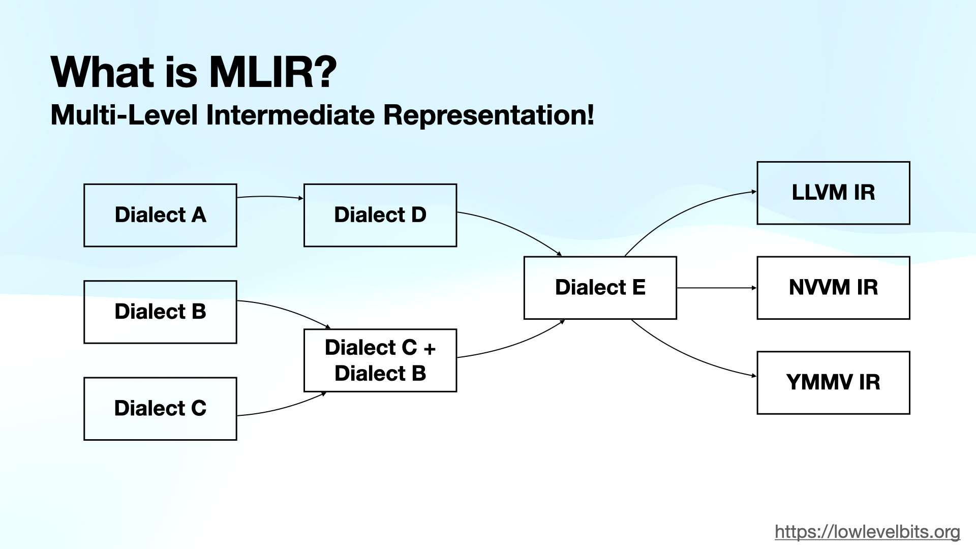
One of the key features of MLIR is the ability to define custom intermediate representations called dialects. MLIR provides an infrastructure to mix and match different dialects and run analyses or transformations against them. Further, the dialects can be lowered to machine code (e.g., for CPU or GPU).

Here is a slide from my LLVM Social talk to illustrate the idea:

MLIR Rite Dialect

I need to define a custom dialect to make MLIR work for my use case. I called it “Rite.” The dialect needs an operation of each RiteVM opcode and some RiteVM types.

Here is the minimum required to compile the code sample from above (puts 42).

def Rite_Dialect : Dialect {
  let name = "rite";
  let summary = "A one-to-one mapping from mruby RITE VM bytecode to MLIR";

  let cppNamespace = "rite";
}

class RiteType<string name> : TypeDef<Rite_Dialect, name> {
  let summary = name;
  let mnemonic = name;
}

def ValueType : RiteType<"value"> {}
def StateType : RiteType<"state"> {}

class Rite_Op<string mnemonic, list<Trait> traits = []> :
    Op<Rite_Dialect, mnemonic, traits>;

// OPCODE(LOADSELF, B) /* R(a) = self */
def LoadSelfOp : Rite_Op<"OP_LOADSELF"> {
  let summary = "OP_LOADSELF";
  let results = (outs ValueType);
}

// OPCODE(LOADI, BB) /* R(a) = mrb_int(b) */
def LoadIOp : Rite_Op<"OP_LOADI"> {
  let summary = "OP_LOADI";
  let arguments = (ins SI64Attr:$value);
  let results = (outs ValueType);
}

// OPCODE(SEND, BBB) /* R(a) = call(R(a),Syms(b),R(a+1),...,R(a+c)) */
def SendOp : Rite_Op<"OP_SEND"> {
  let summary = "OP_SEND";
  let arguments = (ins ValueType:$receiver, StringAttr:$symbol, UI32Attr:$argc, Variadic<ValueType>:$argv);
  let results = (outs ValueType);
}

// OPCODE(RETURN, B) /* return R(a) (normal) */
def ReturnOp : Rite_Op<"OP_RETURN", [Terminator]> {
  let summary = "OP_RETURN";
  let arguments = (ins ValueType:$src);
  let results = (outs ValueType);
}

It defines the dialect, the types needed, and the operations. Some entities come from the MLIR’s predefined dialects (StringAttr, UI32Attr, Variadic<...>, Terminator). We define the rest.

Each operation may take zero or more arguments, but it also may produce zero or more results. Unlike a “typical” programming language, MLIR dialects define a graph (as ins and outs hint at). The dialects also have some other properties, but one step at a time.

With the dialect in place, I can generate an “MLIR program” which is roughly equivalent to the C program above:

Note: I omit some details for brevity.

module @"test.rb" {
  func @top(%arg0: !rite.state, %arg1: !rite.value) -> !rite.value {
    %0 = rite.OP_LOADSELF() : () -> !rite.value
    %1 = rite.OP_LOADI() {value = 42 : si64} : () -> !rite.value
    %2 = rite.OP_SEND(%0, %1) {argc = 1 : ui32, symbol = "puts"} : (!rite.value, !rite.value) -> !rite.value
    %3 = rite.OP_RETURN(%2) : (!rite.value) -> !rite.value
  }
}

Here, I generated an MLIR module containing a function (top) with four operations corresponding to each bytecode operation.

Let’s take a detailed look at one operation:

%2 = rite.OP_SEND(%0, %1) {argc = 1 : ui32, symbol = "puts"} : (!rite.value, !rite.value) -> !rite.value

This piece defines a value named %2, which takes two other values (%0 and %1). In MLIR, constants are defined as “attributes,” which are argc = 1 : ui32 and symbol = "puts" in this case. What follows is the operation signature (!rite.value, !rite.value) -> !rite.value. The operation returns rite.value and takes several arguments: %0 is the receiver, and %1 is part of the Variadic<ValueType>:$argv.

MLIR takes the declarative dialect definition and generates C++ code out of it. The C++ code serves as a programmatic API to generate the MLIR module.

Once the module is generated, I can analyze and transform it. The next step is directly converting the Rite Dialect into LLVM Dialect and lowering it into LLVM IR.

From there on, I can emit an object file (machine code) and link it with mruby runtime.

Static Single Assignment (SSA)

In the previous article, I mentioned that the virtual stack is essential, yet here in both C and MLIR programs, I use “local variables” instead of the stack. What’s going on here?

The answer is simple - MLIR uses a Static Single-Assignment form for all its representations.

As a reminder, SSA means that each variable can only be defined once.

Pedantic note: the “variables” should be referred to as “values” as they cannot vary.

Here is an “invalid” SSA form:

int x = 42;
x = 55; // redefinition not allowed in SSA
print(x);

And here is the same code in the SSA form:

int x = 42;
int x1 = 55; // "redefinition" generates a new value
print(x1);

We must convert the registers into SSA values to satisfy the MLIR requirement to be in SSA form.

At first glance, the problem is trivial. We can maintain a map of definitions for each register at each point in time. For example, for the following bytecode:

OP_LOADSELF R1    // #1
OP_LOADI    R2 10 // #2
OP_LOADI    R3 20 // #3
OP_LOADI    R3 30 // #4
OP_ADD      R2 R3 // #5
OP_RETURN   R2    // #6

The map changes as follows:

Step #1: { empty }
Step #2: {
  R1 defined by #1
}
Step #3: {
  R1 defined by #1
  R2 defined by #2
}
Step #4: {
  R1 defined by #1
  R2 defined by #2
  R3 defined by #3
}
Step #5: {
  R1 defined by #1
  R2 defined by #2
  R3 defined by #4 // R3 redefined at #4
}
Step #5: {
  R1 defined by #1
  R2 defined by #5 // OP_ADD stores the result in the first operand
  R3 defined by #4
}

With this map, we know precisely where a register was defined when an operation uses the register.

So MLIR version will look like this:

// OP_LOADSELF R1
%0 = rite.OP_LOADSELF() : () -> !rite.value
// OP_LOADI    R2 10
%1 = rite.OP_LOADI() {value = 10 : si64} : () -> !rite.value
// OP_LOADI    R3 20
%2 = rite.OP_LOADI() {value = 20 : si64} : () -> !rite.value
// OP_LOADI    R3 30
%3 = rite.OP_LOADI() {value = 30 : si64} : () -> !rite.value
// OP_ADD      R2 R3
%4 = rite.OP_ADD(%1, %3) : (!rite.value, !rite.value) -> !rite.value
// OP_RETURN   R2
%5 = rite.OP_RETURN(%4) : (!rite.value) -> !rite.value

Side note: %0 and %2 are never used and can be eliminated (if OP_LOADSELF/OP_LOADI don’t have side effects).

This solution is pleasant until the code has branching such as if/else, loops, or exceptions.

Consider the following non-SSA example:

x = 10;
if (something) {
  x = 20;
} else {
  x = 30;
}
print(x); // Where x is defined?

Classical SSA solves this problem with artificial phi-nodes:

x1 = 10;
if (something) {
  x2 = 20;
} else {
  x3 = 30;
}
x4 = phi(x2, x3); // Will magically resolve to the right x depending on where it comes from
print(x4);

MLIR approaches this differently and elegantly - via “block arguments.”

But first, let’s talk about Control-Flow Graphs.

Control-Flow Graph (CFG)

A control-flow graph is a form of intermediate representation that maintains the program in the form of a graph where operations are connected to each other based on the execution (or control) flow.

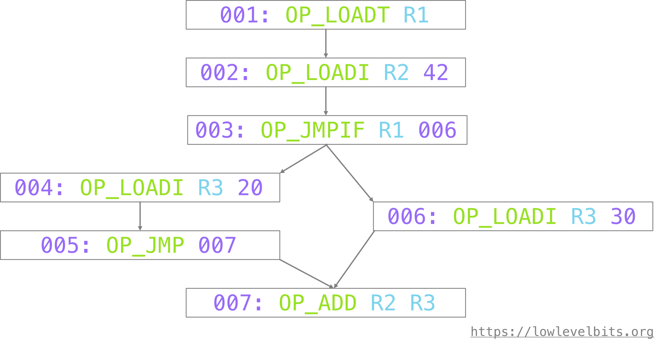
Consider the following bytecode (the number on the left is an operation address):

001: OP_LOADT R1      // puts "true" in R1
002: OP_LOADI R2 42
003: OP_JMPIF R1 006  // jump to 006 if R1 contains "true"
                      // otherwise implicitly falls through to 004
004: OP_LOADI R3 20
005: OP_JMP 007       // jump to 007 unconditionally
006: OP_LOADI R3 30
007: OP_ADD R2 R3     // R3 may be either 20 or 30, depending on the branching

The same program in the form of a graph:

This CFG can be further optimized: we can merge all the subsequent nodes unless the node has more than one incoming or more than one outgoing edge.

The merged nodes are called basic blocks:

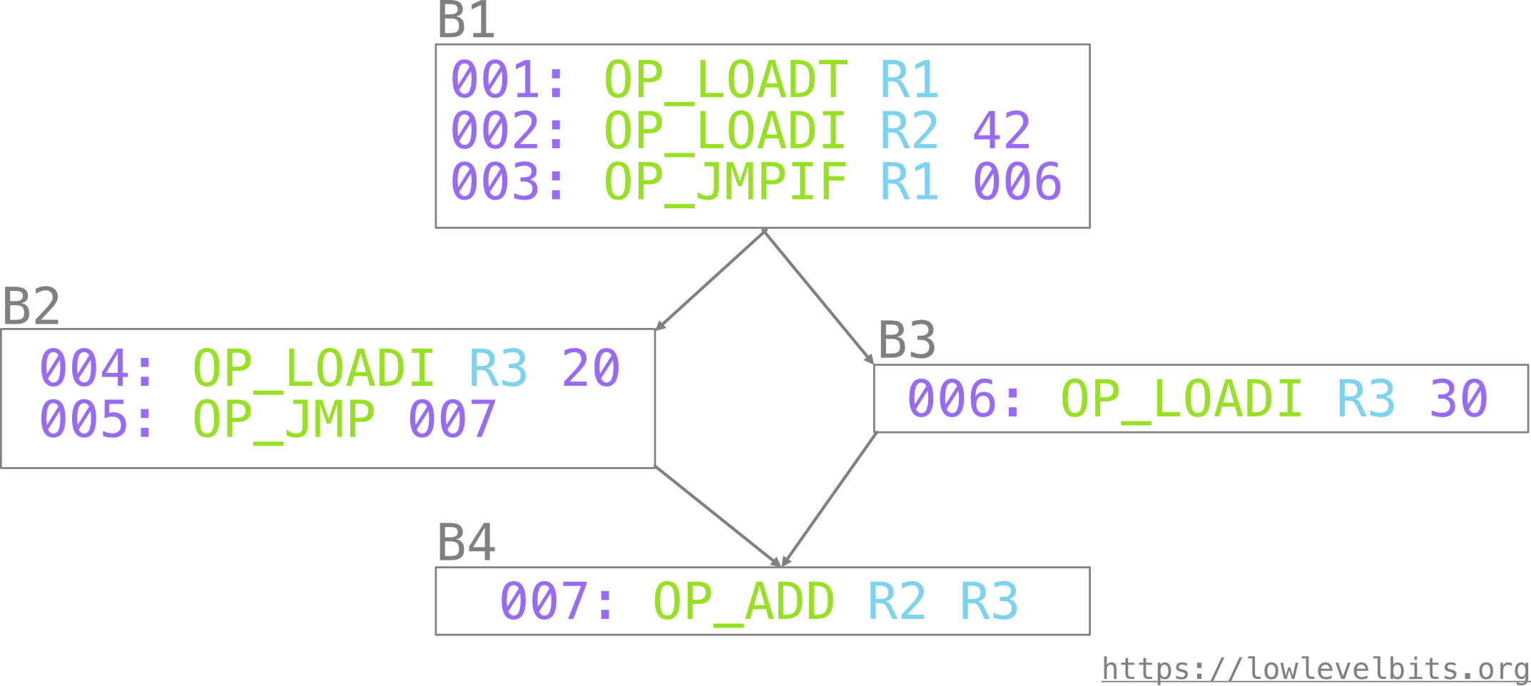
Some more terms for completeness:

• the “first” basic block where the execution of a function starts is called “entry.”
• similarly, the “last” basic block is called “exit.”
• preceding (incoming, previous) basic blocks are called predecessors. The entry block doesn’t have predecessors.
• succeeding (outgoing, next) basic blocks are called successors. Exit blocks don’t have successors.
• the last operation in a basic block is called a terminator

Based on the last picture:

• B1: entry block
• B4: single exit block. There could be several exit blocks, yet we can always add one “empty” block as a successor for the exit blocks to have only one exit block.
• B1: predecessors: [], successors: [B2, B3], terminator: OP_JMPIF
• B2: predecessors: [B1], successors: [B4], terminator: OP_JMP
• B3: predecessors: [B1], successors: [B4], terminator: OP_LOADI
• B4: predecessors: [B2, B3], successors: [], terminator: OP_ADD

CFGs in MLIR

Now we can take a look at CFGs from the MLIR perspective. If you are familiar with CFGs in LLVM, then the important difference is that in MLIR, all the basic blocks may have arguments. Function arguments are, in fact, the block arguments from the entry block. For example, this is a more accurate representation of a function:

func @top() -> !rite.value {
^bb0(%arg0: !rite.state, %arg1: !rite.value):
  %0 = rite.OP_LOADSELF() : () -> !rite.value
  %1 = rite.OP_LOADI() {value = 42 : si64} : () -> !rite.value
  %2 = rite.OP_SEND(%0, %1) {argc = 1 : ui32, symbol = "puts"} : (!rite.value, !rite.value) -> !rite.value
  %3 = rite.OP_RETURN(%2) : (!rite.value) -> !rite.value
}

Note, ^bbX represents the basic blocks.

To convert the following bytecode:

001: OP_LOADT R1      // puts "true" in R1
002: OP_LOADI R2 42
003: OP_JMPIF R1 006  // jump to 006 if R1 contains "true"
                      // otherwise implicitly falls through to 004
004: OP_LOADI R3 20
005: OP_JMP 007       // jump to 007 unconditionally
006: OP_LOADI R3 30
007: OP_ADD R2 R3     // R3 may be either 20 or 30, depending on the branching

we need to take several steps:

• add an address attribute to all addressable operations (they could be jump targets)
• add “targets” attribute to all the jumps, including implicit fallthrough jumps
• add an explicit jump in place of the implicit jumps
• add the successor blocks for all jump instructions
• put all the operations in a single, entry basic block

func @top(%arg0: !rite.state, %arg1: !rite.value) -> !rite.value {
  %0 = rite.PhonyValue() : () -> !rite.value
  %1 = rite.OP_LOADT() { address = 001 } : () -> !rite.value
  %2 = rite.OP_LOADI() { address = 002, value = 42 } : () -> !rite.value
  rite.OP_JMPIF(%0)[^bb1, ^bb1] { address = 003, targets = [006, 004] }
  %3 = rite.OP_LOADI() { address = 004, value = 20 } : () -> !rite.value
  rite.OP_JMP()[^bb1] { address = 005, targets = [007] }
  %4 = rite.OP_LOADI() { address = 006, value = 30 } : () -> !rite.value
  rite.FallthroughJump()[^bb1]
  %5 = rite.OP_ADD(%0, %0) { address = 007 } : () -> !rite.value
^bb1:
}

Note: I’m omitting some details from the textual representation for brevity.

Notice, here, I added a “phony value” as a placeholder for SSA values as we cannot yet construct the proper SSA. We will remove them in the next section.

Additionally, I added a phony basic block to serve as a placeholder successor for the jump targets.

Now, the last steps are:

• split the entry basic block by cutting it right before each jump target operation
• rewire the jumps to point to the right target basic blocks
• delete the phony basic block used as a placeholder

The final CFG looks like this:

func @top(%arg0: !rite.state, %arg1: !rite.value) -> !rite.value {
  %0 = rite.PhonyValue() : () -> !rite.value
  %1 = rite.OP_LOADT() { address = 001 } : () -> !rite.value
  %2 = rite.OP_LOADI() { address = 002, value = 42 } : () -> !rite.value
  rite.OP_JMPIF(%0)[^bb1, ^bb2] { address = 003, targets = [006, 004] }
^bb1: // pred: ^bb0
  %3 = rite.OP_LOADI() { address = 004, value = 20 } : () -> !rite.value
  rite.OP_JMP()[^bb3] { address = 005, targets = [007] }
^bb2: // pred: ^bb0
  %4 = rite.OP_LOADI() { address = 006, value = 30 } : () -> !rite.value
  rite.FallthroughJump()[^bb3]
^bb3: // pred: ^bb1, ^bb2
  %5 = rite.OP_ADD(%0, %0) { address = 007 } : () -> !rite.value
}

It corresponds to the last picture above, except that we now have an explicit rite.FallthroughJump().

With the CFG in place, we can solve the SSA problem and eliminate the rite.PhonyValue() placeholder.

SSA in MLIR

As a reminder, here is the CFG of the “problematic” program:

In the MLIR form, we no longer have registers from the virtual stack. We only have values such as %2, %3, %4, and so on. The tricky part is the 007: OP_ADD R2 R3 operation - where R3 is coming from? Is it %3 or %4?

To answer this question, we can use Data-flow analysis.

Dataflow analysis is used to derive specific facts about the program. The analysis is an iterative process: first, collect the base facts for each basic block, then for each basic block, update the facts combining them with the facts from successors or predecessors. As the facts updated for a basic block may affect the facts from successors/predecessors, the process should run iteratively until no new facts are derived.

A critical requirement for the facts - they should be monotonic. Once the fact is known, it cannot “disappear.” This way, the iterative process eventually stops as, in the worst case, the analysis will derive “all” the facts about the program and won’t be able to derive any more.

My favorite resource about dataflow analysis is Adrian Sampson’s lectures on the subject - The Data Flow Framework. I highly recommend it.

In our case, the facts we need to derive are: which values/registers are required for each operation.

Here is an algorithm briefly:

• at every point in time, there is a map of the values defined so far
• if an operation is using a value that is not defined, then this value is required
• the required values become the block arguments and must be coming from the predecessors
• the terminators of the “required” predecessors now use the values required by the successors
• at the next iteration, the block arguments define the previously required values

The process runs iteratively until no new required values appear.

An important detail for the entry basic block is that, as it doesn’t have a predecessor, all the required values must come from the virtual stack.

Let’s look a the example bytecode once again:

001: OP_LOADT R1
002: OP_LOADI R2 42
003: OP_JMPIF R1 006
004: OP_LOADI R3 20
005: OP_JMP   007
006: OP_LOADI R3 30
007: OP_ADD   R2 R3

This is the initial state for the dataflow analysis. The comments above contain information about defined values for the given point in time. Comment on the side of each operation tells about the operation itself:

func @top(%arg0: !rite.state, %arg1: !rite.value) -> !rite.value {
  // defined: []
  %0 = rite.PhonyValue() : () -> !rite.value   // defines: [], uses: []
  // defined: []
  %1 = rite.OP_LOADT() : () -> !rite.value     // defines: [R1], uses: []
  // defined: [R1]
  %2 = rite.OP_LOADI(42) : () -> !rite.value   // defines: [R2], uses: []
  // defined: [R1, R2]
  rite.OP_JMPIF(%0)[^bb1, ^bb2]                // defines: [], uses: [R1]

^bb1: // pred: ^bb0                            // defines: [], uses: []
  // defined: []
  %3 = rite.OP_LOADI(20) : () -> !rite.value   // defines: [R3], uses: []
  // defined: [R3]
  rite.OP_JMP()[^bb3]                          // defines: [], uses: []

^bb2: // pred: ^bb0                            // defines: [], uses: []
  // defined: []
  %4 = rite.OP_LOADI(30) : () -> !rite.value   // defines: [R3], uses: []
  // defined: [R3]
  rite.FallthroughJump()[^bb3]                 // defines: [], uses: []

^bb3: // pred: ^bb1, ^bb2                      // defines: [], uses: []
  // defined: []
  %5 = rite.OP_ADD(%0, %0) : () -> !rite.value // defines: [R2], uses: [R2, R3]
}

The last operation uses values that are not defined. Therefore R2 and R3 are required and must come from the predecessors.

Update predecessors and rerun the analysis.

Note: I am using %RX_Y names to distinguish them from the original numerical value names. X is the register number, and Y is the basic block number.

func @top(%arg0: !rite.state, %arg1: !rite.value) -> !rite.value {
  // defined: []
  %0 = rite.PhonyValue() : () -> !rite.value   // defines: [], uses: []
  // defined: []
  %1 = rite.OP_LOADT() : () -> !rite.value     // defines: [R1], uses: []
  // defined: [R1]
  %2 = rite.OP_LOADI(42) : () -> !rite.value   // defines: [R2], uses: []
  // defined: [R1, R2]
  rite.OP_JMPIF(%0)[^bb1, ^bb2]                // defines: [], uses: [R1]

^bb1: // pred: ^bb0                            // defines: [], uses: []
  // defined: []
  %3 = rite.OP_LOADI(20) : () -> !rite.value   // defines: [R3], uses: []
  // defined: [R3]
  rite.OP_JMP(%0, %0)[^bb3]                    // defines: [], uses: [R2, R3]

^bb2: // pred: ^bb0                            // defines: [], uses: []
  // defined: []
  %4 = rite.OP_LOADI(30) : () -> !rite.value   // defines: [R3], uses: []
  // defined: [R3]
  rite.FallthroughJump(%0, %0)[^bb3]           // defines: [], uses: [R2, R3]

^bb3(%R2_3, %R3_3): // pred: ^bb1, ^bb2        // defines: [R2, R3], uses: []
  // defined: [R2, R3]
  %5 = rite.OP_ADD(%0, %0) : () -> !rite.value // defines: [R2], uses: [R2, R3]
}

Basic block ^bb3 now has two block arguments. The terminators from its predecessors (^bb1 and ^bb2) now use an undefined value, R2. R2 is now required. We must add it as a block argument and propagate it to the predecessors’ terminators.

Rerun the analysis:

func @top(%arg0: !rite.state, %arg1: !rite.value) -> !rite.value {
  // defined: []
  %0 = rite.PhonyValue() : () -> !rite.value   // defines: [], uses: []
  // defined: []
  %1 = rite.OP_LOADT() : () -> !rite.value     // defines: [R1], uses: []
  // defined: [R1]
  %2 = rite.OP_LOADI(42) : () -> !rite.value   // defines: [R2], uses: []
  // defined: [R1, R2]
  rite.OP_JMPIF(%0, %0, %0)[^bb1, ^bb2]        // defines: [], uses: [R1, R2, R2]

^bb1(%R2_1): // pred: ^bb0                     // defines: [R2], uses: []
  // defined: [R2]
  %3 = rite.OP_LOADI(20) : () -> !rite.value   // defines: [R3], uses: []
  // defined: [R2, R3]
  rite.OP_JMP(%0, %0)[^bb3]                    // defines: [], uses: [R2, R3]

^bb2(%R2_2): // pred: ^bb0                     // defines: [R2], uses: []
  // defined: [R2]
  %4 = rite.OP_LOADI(30) : () -> !rite.value   // defines: [R3], uses: []
  // defined: [R2, R3]
  rite.FallthroughJump(%0, %0)[^bb3]           // defines: [], uses: [R2, R3]

^bb3(%R2_3, %R3_3): // pred: ^bb1, ^bb2        // defines: [R2, R3], uses: []
  // defined: [R2, R3]
  %5 = rite.OP_ADD(%0, %0) : () -> !rite.value // defines: [R2], uses: [R2, R3]
}

We can run the analysis one more time, but it won’t change anything, so that would conclude the analysis, and we should have all the information we need to replace the phony value with the correct values.

Additionally, now we can replace our custom jump operations with the builtin ones from MLIR, so the final function looks like this:

func @top(%arg0: !rite.state, %arg1: !rite.value) -> !rite.value {
  %1 = rite.OP_LOADT() : () -> !rite.value
  %2 = rite.OP_LOADI(42) : () -> !rite.value
  cond_br %1, ^bb1(%2), ^bb2(%2)
^bb1(%R2_1): // pred: ^bb0
  %3 = rite.OP_LOADI(20) : () -> !rite.value
  br ^bb3(%R2_1, %3)
^bb2(%R2_2): // pred: ^bb0
  %4 = rite.OP_LOADI(30) : () -> !rite.value
  br ^bb3(%R2_2, %4)
^bb3(%R2_3, %R3_3): // pred: ^bb1, ^bb2
  %5 = rite.OP_ADD(%R2_3, %R3_3) : () -> !rite.value
}

Now, onto drawing the rest of the fu**ing owl.

Thank you so much for reaching this far!

The next article gives a short progress update.